How a Large Language Model works

🧠 1. What is a Large Language Model?

A Large Language Model (LLM) is a neural network trained to predict the most likely next word (or token) given everything that came before it. That's it. The surprising thing is that a single objective — predict the next token — turns out to be enough to learn grammar, facts, reasoning patterns, and even code, if you train on enough text.

Modern LLMs are built on the Transformer architecture (introduced by Google in 2017). A Transformer stacks many identical layers, each of which applies a mechanism called self-attention to find relationships between all tokens in the current context simultaneously.

The pipeline from text to answer involves four conceptually distinct stages: tokenize → embed → process → generate. The rest of this page explains each one.

✂️ 2. Tokenization — text becomes numbers

Neural networks can only process numbers, so the first step is converting text into a sequence of integers called token IDs. A tokenizer splits the input string into tokens — units that may be whole words, sub-words, or single characters — and maps each to an integer from a fixed vocabulary.

Real LLMs: Byte-Pair Encoding (BPE)

Most modern LLMs use BPE or a variant (SentencePiece, WordPiece). BPE starts with a vocabulary of individual bytes and repeatedly merges the most frequent adjacent pair. This lets the tokenizer handle any input (it can always fall back to byte-level) while keeping common words as single tokens.

Why sub-word tokenization?

Pure word-based tokenizers fail on rare words and typos. Character-based tokenizers produce very long sequences and slow down training. Sub-word tokenization is the sweet spot: common words are one token, rare words are split into familiar sub-parts.

🔢 3. Embeddings — numbers become vectors

A token ID like 2963 is just an index. Before the Transformer can work with it, each ID is converted into a dense vector (a list of floating-point numbers, typically 768–8192 dimensions) called an embedding.

Think of an embedding as a point in a very high-dimensional space. The training process arranges these points so that semantically similar tokens end up nearby: "king" and "queen" are close; "banana" and "circuit" are far apart.

👁️ 4. Attention — context shapes meaning

The core innovation of the Transformer is self-attention. At each layer, every token looks at every other token and decides how much it should "attend to" them when building its own representation.

Concretely: for each token, three vectors are computed — Query (Q), Key (K), and Value (V). Attention scores are the dot product of Q with all K vectors, normalised by softmax. The output is a weighted sum of V vectors.

In plain English: "The word 'it' in 'The animal was tired because it…' attends strongly to 'animal', so the model represents 'it' as meaning 'the animal'." Attention allows the model to resolve such references regardless of how far apart the tokens are.

Multi-head attention

In practice, attention is computed h times in parallel with different learned projections (the "heads"). Each head can specialise in a different type of relationship: one might track syntax, another coreference, another semantic similarity. The outputs of all heads are concatenated and projected back to the model dimension.

⚡ 5. The generation loop — one token at a time

LLMs generate text autoregressively: one token at a time, each new token conditioned on everything generated so far.

🌡️ 6. Softmax & temperature — shaping the distribution

After the forward pass, the model has a raw score (logit) for every token in the vocabulary. Softmax converts those scores into a proper probability distribution: all values become positive and sum to exactly 1.

What does temperature do?

Temperature T is applied as a divisor before the exponential:

• T = 1.0 — the model's learned distribution, unchanged.
• T < 1 — sharpens the distribution; the top token becomes even more dominant. More deterministic, less creative.
• T > 1 — flattens the distribution; gives more probability mass to unlikely tokens. More diverse, more "creative" (and more likely to be wrong).
• T → 0 — greedy decoding: always picks the single most probable token.

Here's an example showing how temperature changes a concrete distribution:

Other sampling strategies

Temperature is often combined with:

• Top-k sampling — only sample from the k most probable tokens (discard everything else).
• Top-p (nucleus) sampling — only sample from the smallest set of tokens whose cumulative probability exceeds p (e.g. 0.9).
• Repetition penalty — reduce the score of tokens that already appeared in the context, to discourage repetitive output.

🤖 7. Agents & tool use

A bare LLM is a text-in / text-out function. It cannot browse the web, run code, or call an API. Agents extend LLMs with the ability to use tools and take multi-step actions.

How tool use works in real systems

Modern frameworks (OpenAI function calling, Anthropic tool use) work roughly like this:

1. A list of available tools (name, description, JSON schema of parameters) is prepended to the system prompt.
2. The LLM is fine-tuned to output a structured JSON block when it decides a tool is needed (instead of plain text).
3. The host application parses that JSON, calls the real tool, and inserts the result back into the conversation as a new message.
4. The LLM continues generating from there, now with the tool result in its context.

Chain-of-thought reasoning

Before deciding which tool to call (or whether to call one at all), frontier models often produce a reasoning trace — a scratchpad of intermediate thoughts. In the OpenAI "o" series and DeepSeek-R1, this trace is explicit and inspectable. In older models it was hidden or only possible via prompting ("Let's think step by step").

🔬 8. What this simulation actually does

The full pipeline, from the moment you hit Ask → to the moment the trace is ready:

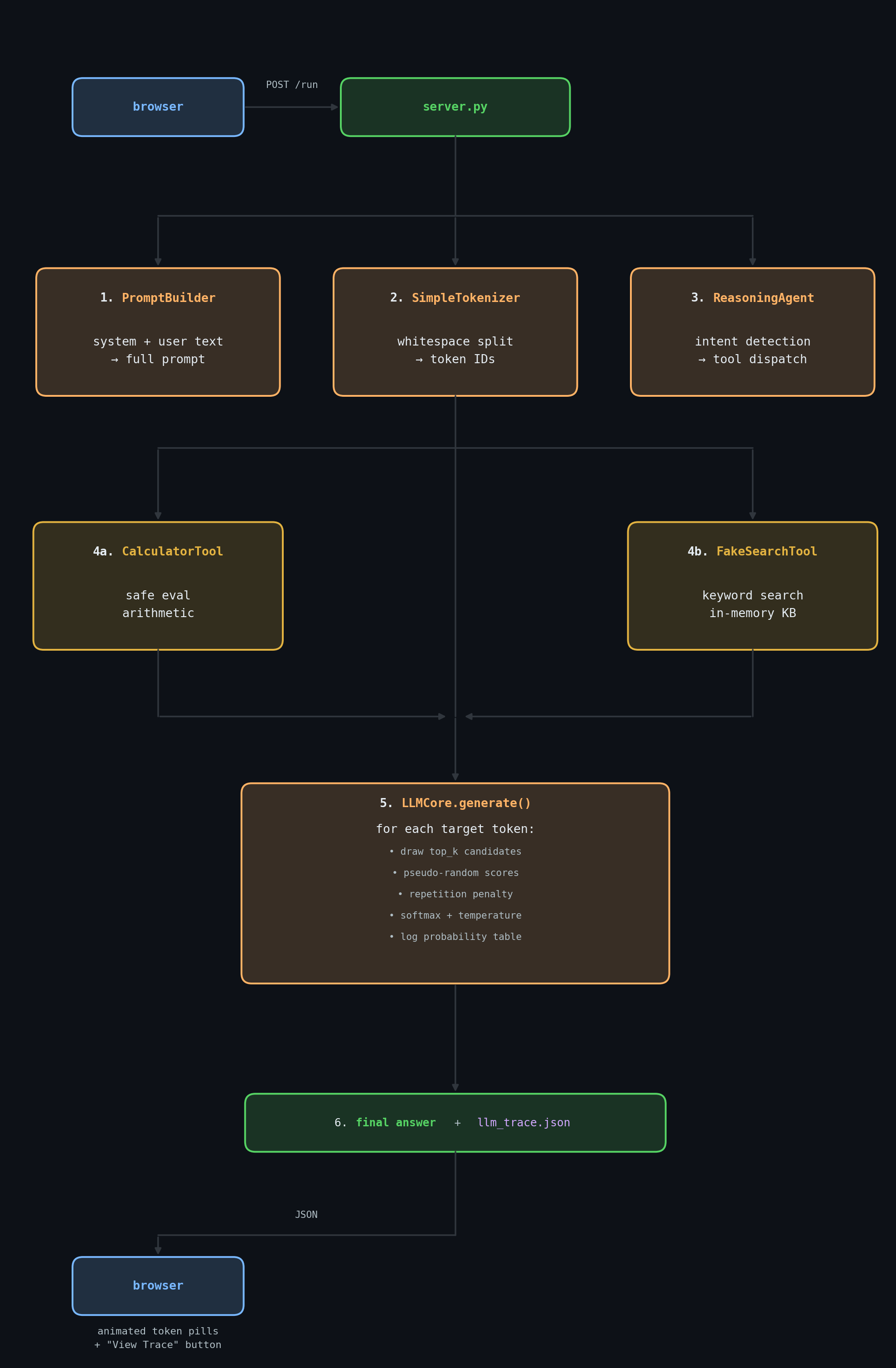
Every one of these steps writes a TraceStep into the append-only Trace object. At the end the trace is serialised to llm_trace.json and served at GET /llm_trace.json. The Trace Viewer fetches it and renders every step as an expandable card.

Real vs. simulated — side by side

⚠️ 9. What this simulation cannot show

This project is deliberately simplified for educational purposes. Here are the most important things that are not represented:

• Emergent capabilities — the ability to translate, reason about logic, write code, etc. comes from training on enormous datasets with billions of parameters, not from the architecture alone.
• RLHF / RLAIF — modern assistants (ChatGPT, Claude) are fine-tuned with reinforcement learning from human (or AI) feedback, which fundamentally shapes tone, safety, and instruction-following.
• True semantic understanding — the simulation's token scores are random; a real model's scores encode the statistical regularities of human language.
• KV-cache — real inference reuses the key/value tensors from previous tokens to avoid re-computing the full forward pass at every step (huge performance win). Not relevant here since there is no forward pass.
• Quantization & hardware — running a 70B model requires tens of GB of VRAM. Techniques like 4-bit quantization (GGUF) and speculative decoding are critical in practice.